class: center, middle, inverse, title-slide # Topic 4: Spatial Point Patterns Analysis ### Dr. Kam Tin Seong<br/>Assoc. Professor of Information Systems (Practice) ### School of Computing and Information Systems,<br/>Singapore Management University ### 2020-5-5 (updated: 2021-05-17) --- # Content .large[ - Introducing Spatial Point Patterns - The basic concepts of spatial point patterns - 1st Order versus 2nd Order - Spatial Point Patterns in real world - 1st Order Spatial Point Patterns Analysis - Quadrat analysis - Kernel density estimation - 2nd Order Spatial Point Patterns Analysis - Nearest Neighbour Index - G-function - F-function - K-function - L-function ] --- # What is Spatial Point Patterns .large[ - Points as Events - Mapped pattern - Not a sample - Selection bias - Events are mapped, but non-events are not ] --- ## Spatial Point Patterns in Real World .large[ - Distribution of dieses such as dengue fever.] .center[ ] --- ## Spatial Point Patterns in Real World .large[ - Distribution of car collisions.] .center[ ] --- ## Spatial Point Patterns in Real World .large[ - Distribution of crime incidents.] .center[ ] --- ## Spatial Point Patterns in Real World .large[ - Distribution of public services such as education institutions.] .center[ ] --- ## Spatial Point Patterns in Real World .large[ - Locations of the different channel stores.] .center[ ] --- ## Spatial Point Patterns in Real World .large[ - Distribution of social media data such as tweets.] .center[ ] --- # Real World Question .large[ - Location only - are points randomly located or patterned - Location and value - marked point pattern - is combination of location and value random or patterned - What is the underlying process? ] --- ## Points on a Plane .large[ - Classic point pattern analysis - points on an isotropic plane - no effect of translation and rotation - classic examples: tree seedlings, rocks, etc - Distance - straight line only] --- ## Real world spatial point patterns .large[ - Is this a random distribution?] .center[ ] --- ## Real world spatial point patterns .large[ - Is this a random distribution?] .center[ ] --- # Spatial Point Patterns Analysis .large[ - Point pattern analysis (PPA) is the study of the spatial arrangements of points in (usually 2-dimensional) space. - The simplest formulation is a set X = {x ∈ D} where D, which can be called the **study region**, is a subset of Rn, a n-dimensional **Euclidean space**. - A fundamental problem of PPA is inferring whether a given arrangement is merely **random** or the result of some process.] .center[ ] --- # Spatial Point Patterns Analysis Techniques .large[ - First-order vs Second-order Analysis of spatial point patterns.] .center[ ] .small[Reference: 11.4 First and second order effects of Intro to GIS and Spatial Analysis (https://mgimond.github.io/Spatial/point-pattern-analysis.html#first-and-second-order-effects) ] ??? The first-order properties describe the way in which the expected value (mean or average) of the spatial point pattern varies across space (i.e., the intensity of the spatial point pattern). Such properties are usually measured with the so-called quadrat analysis, nearest neighbour index and kernel estimation. Second-order properties describe the covariance (or correlation) between values of the spatial point pattern at different regions in space and are usually measured with the G function, K function and L function. Applied to point event data, both properties could be used to explore the spatial variation in the risk of being victimized by a crime, spatial and space-time clustering of criminal activities, and the raised incidence of criminal activities around point sources, such as robberies around ATM machines, subway entrances and exits, etc. --- ## First-order Spatial Point Patterns Analysis Techniques .large[ - Density-based - Quadrat analysis, - Kernel density estimation - Distance-based - Nearest Neighbour Index ] --- ## Basic concept of density-based measures .center[ ] --- ### Quadrat Analysis – Step 1 .large[ - Divide the study area into subregion of equal size, - often squares, but don’t have to be.] .center[ ] --- ### Quadrat Analysis – Step 2 .large[ - Count the frequency of events in each region.] .center[ ] --- ### Quadrat Analysis – Step 3 .large[ - Calculate the intensity of events in each region.] .center[ ] --- ### Quadrat Analysis – Step 4 .large[ - Calculate the quadrat statistics and perform CSR test.] .center[ ] --- ### Quadrat Analysis – Variance-Mean Ratio (VMR) .large[ - For an **uniform** distribution, the variance is zero, - therefore, we expect a variance-mean ratio **close to 0**. - For a **random** distribution, the variance and mean are the same, - therefore, we expect a variance-mean ratio **close to 1**. - For a **cluster** distribution, the variance is relatively large, - therefore, we expect a variance-mean ratio **greater than 1**.] --- ### Complete Spatial Randomness (CSR) .pull-left[ .large[ - CSR/IRP satisfy two conditions: - Any event has equal probability of being in any location, a **1st order** effect. - The location of one event is independent of the location of another event, a **2nd order** effect. ] .small[Reference: Source: Chapter 12 Hypothesis testing of Intro to GIS and Spatial Analysis (https://mgimond.github.io/Spatial/hypothesis-testing.html) ]] .pull-right[ ] --- ### Quandrat Analysis: The interpretation .center[ 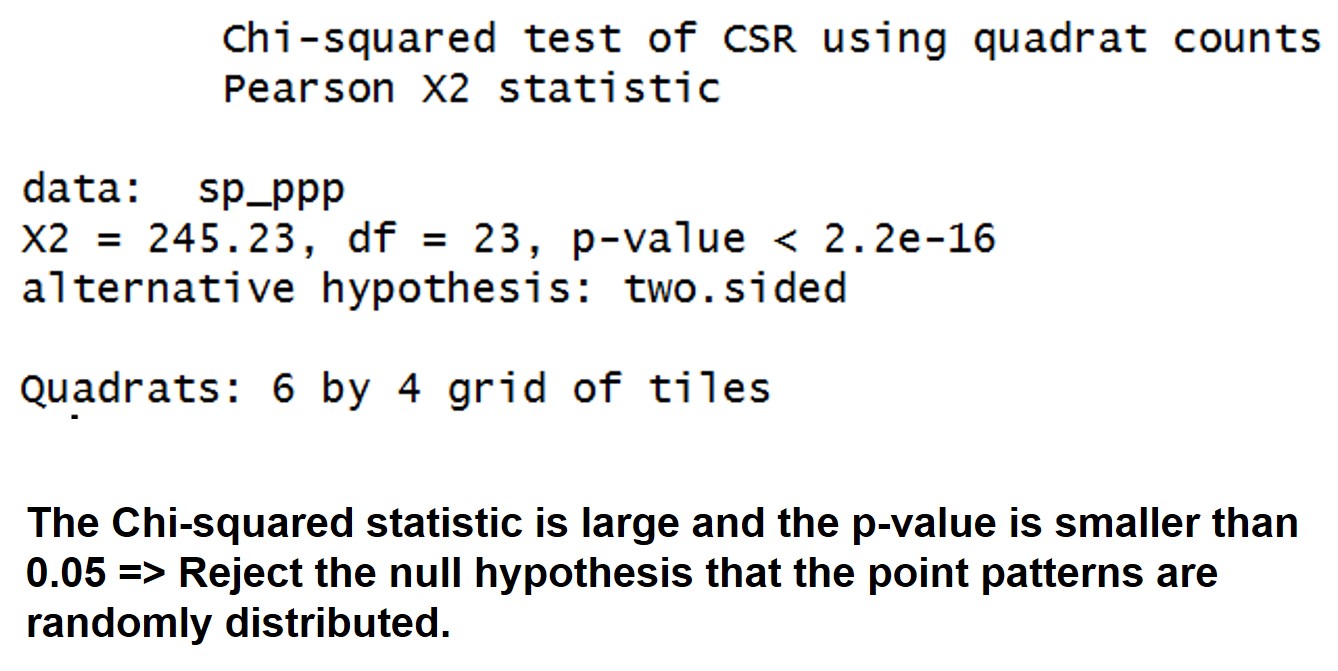] --- ### Weaknesses of quadrat analysis .pull-left[ .large[ - It is sensitive to the quadrat size. - If the quadrat size is too small, they may contain only a couple of points, and - If the quadrat size is too large, they may contain too many points. - It is a measure of **dispersion** rather than a measure of **pattern**. - It results in a single measure for the entire distribution, so variation within the region are not recognised.]] .pull-right[ 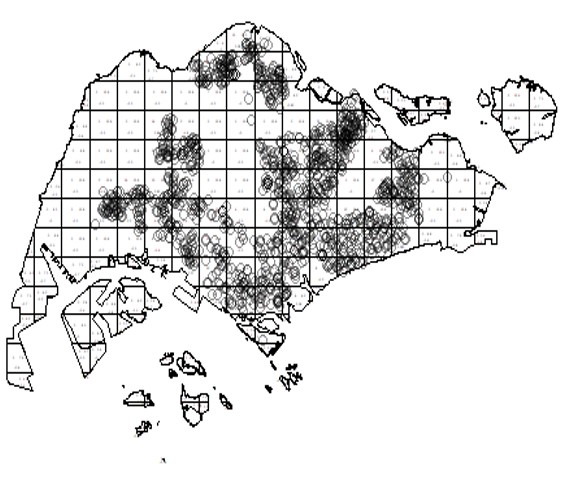] --- ## Distance-based: Nearest Neighbour Index ### What is Nearest Neighbour? .large[ Direct distance from a point to its nearest neighbour.] .center[ 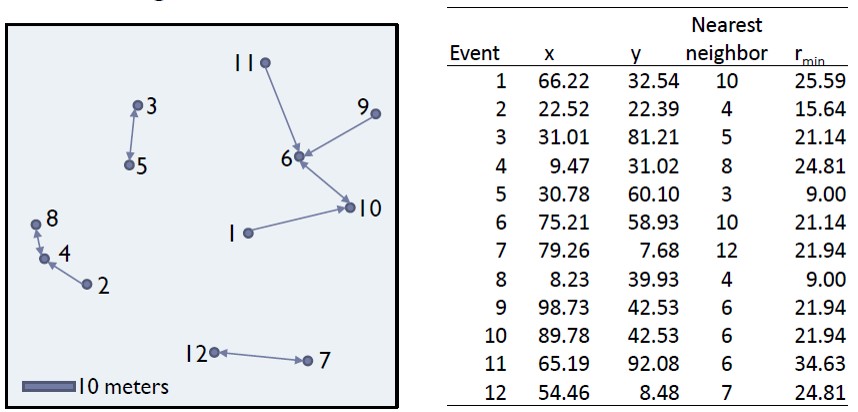] --- ## Nearest Neighbour Index .large[ The Nearest Neighbour Index is expressed as the ratio of the **Observed Mean Distance** to the **Expected Mean Distance**.] .center[ 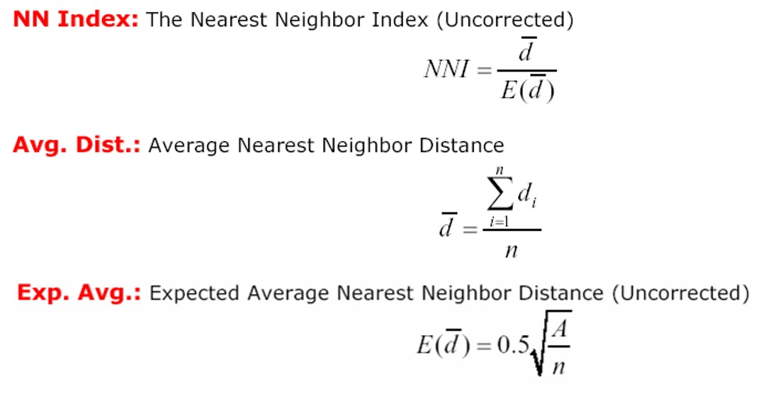] --- ### Calculating Nearest Neighbour Index .center[ ] --- ### Interpreting Nearest Neighbour Index .large[ The expected distance is the average distance between neighbours in a hypothetical random distribution. - If the index is less than 1, the pattern exhibits clustering, - If the index is equal to 1, the patterns exhibits random, and - If the index is greater than 1, the trend is toward dispersion or competition.] .center[ ] --- ### The test statistics .large[ - Null Hypothesis: Points are randomly distributed - Test statistics:] .center[ ] .large[ - Reject the null hypothesis if the z-score is large and p-value is smaller than the alpha value.] --- ### Interpreting Nearest Neighbour Index .center[ ] .large[ The p-value is smaller than 0.05 => Reject the null hypothesis that the point patterns are randomly distributed.] --- ## G function .pull-left[ .large[ The formula] 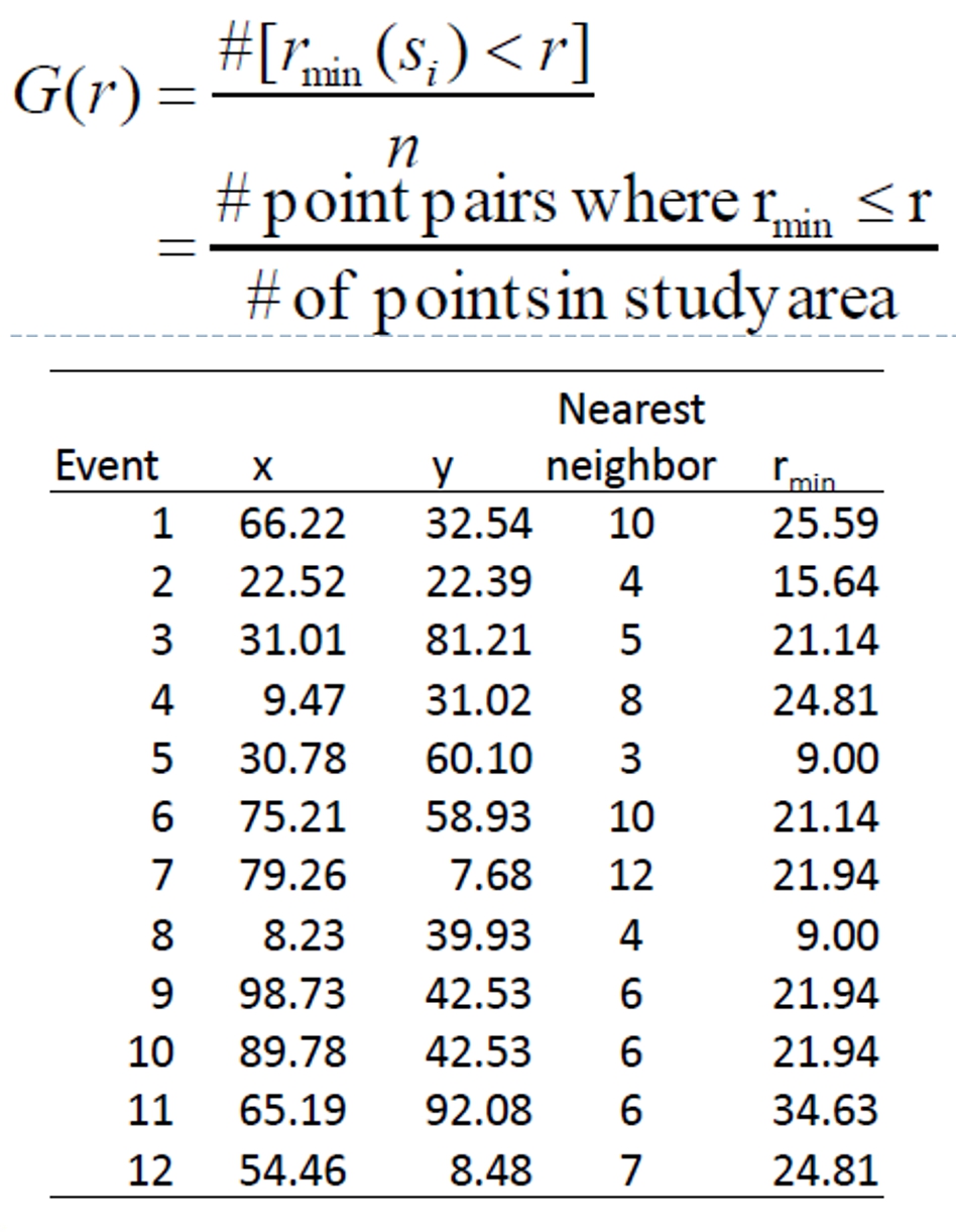] .pull-right[ 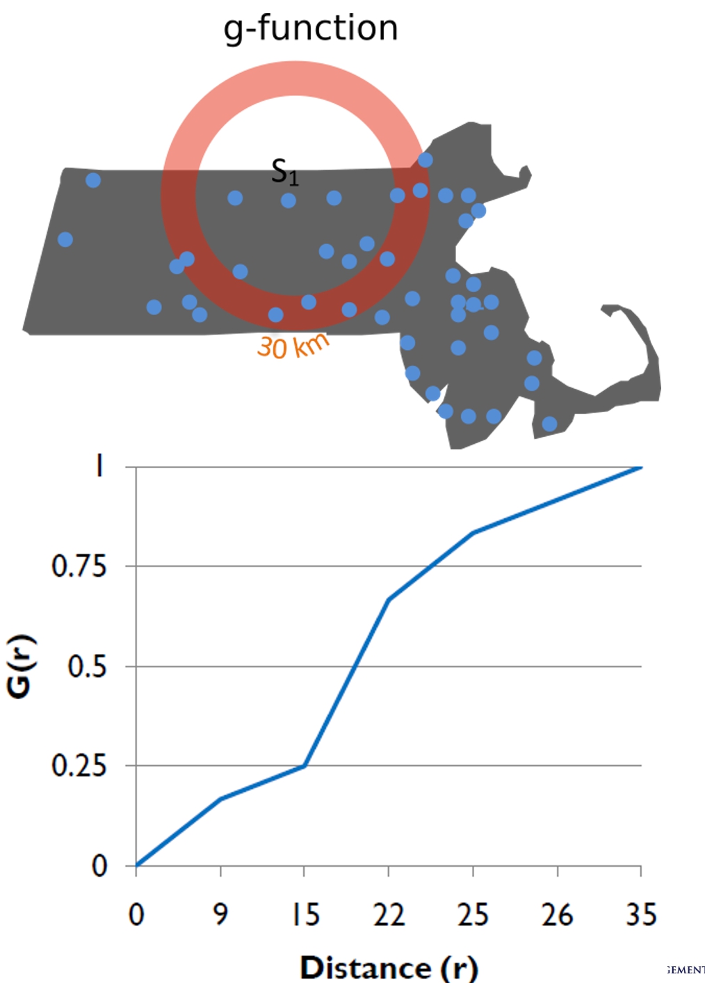] --- ### Interpretation of G-function .pull-left[ .large[ The shape of G-function tells us the way the events are spaced in a point pattern. - Clustered = G increases rapidly at short distance. - Evenness = G increases slowly up to distance where most events spaced, then increases rapidly. ]] .pull-right[ 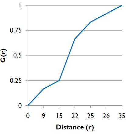] --- ### How do we tell if G is significant? .large[ .pull-left[ - The significant of any departure from CSR (either cluster or regularity) can be evaluated using simulated “confidence envelopes”]] .pull-right[ 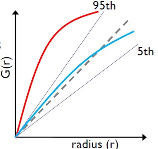] --- ### Monte Carlo simulation test of CSR .large[ - Perform m independent simulation of n events (i.e. 999) in the study region. - For each simulated point pattern, estimate G(r) and use the maximum (95th) and minimum (5th) of these functions for the simulated patterns to define an upper and lower simulation envelope. - If the estimated G(r) lies above the upper envelope or below the lower envelope, the estimated G(r) is statistically significant. ] --- ### The significant test of G-function .center[ ] --- ## F function .large[ - Select a sample of point locations anywhere in the study region at random - Determine minimum distance from each point to any event in the study area. - Three steps: - Randomly select m points (p1, p2, ….., pn), - Calculate dmin(pi,s) as the minimum distance from location pi to any event in the point patterns, and - Calculate F(d).] --- ### The F function formula .center[ ] --- ### Interpretation of F-function .large[ - Clustered = F(r) rises slowly at first, but more rapidly at longer distances. - Evenness = F(r) rises rapidly at first, then slowly at longer distances. ] --- ### The significant test of F-function .center[ ] --- ### Comparison between G and F .center[ ] --- ## Ripley’s K function (Ripley, 1981) .large[ - Limitation of nearest neighbor distance method is that it uses only nearest distance - Considers only the shortest scales of variation. - K function uses more points - Provides an estimate of spatial dependence over a wider range of scales. - Based on all the distances between events in the study area. - Assumes isotropy over the region] --- ### Calculating the K function .pull-left[ .large[ - Construct a circle of radius h around each point event(i). - Count the number of other events (j) that fall inside this circle. - Repeat these two steps for all points (i) and sum results. - Increment h by a small amount and repeat the calculation. ]] .pull-right[ ] --- ### K function The formula: .center[  ] --- ### The K function complete spatial randomness test .large[ - K(h) can be plotted against different values of h. - But what should K look like for no spatial dependence? - Consider what K(h) should look like for a random point process (CSR) - The probability of an event at any point in R is independent of what other events have occurred and equally likely anywhere in R ] --- ### Interpreting the K function complete spatial randomness test .pull-left[ .large[ Under the assumption of CSR, the expected number of events within distance h of an event is:  Compare K(h) to 𝜋ℎ^2 - K(h) < 𝜋ℎ^2 if point pattern is regular - K(h) > 𝜋ℎ^2 if point pattern is clustered ]] .pull-right[  .large[ - Above the envelop = significant cluster pattern - Below the envelop = significant regular - Inside the envelop = CSR ]] --- ## The L function (Besag 1977) .large[ In practice, K function will be normalised to obtained a benchmark of zero. The formula: ] .center[ ] --- ### Interpreting the L function complete spatial randomness test .pull-left[ - When an observed L value is greater than its corresponding L(theo)(i.e. red break line) value for a particular distance and above the upper confidence envelop, spatial clustering for that distance is statistically significant (e.g. distance beyond C). - When an observed L value is greater than its corresponding L(theo) value for a particular distance and lower than the upper confidence envelop, spatial clustering for that distance is statistically NOT significant (e.g. distance between B and C). - When an observed L value is smaller than its corresponding L(theo) value for a particular distance and beyond the lower confidence envelop, spatial dispersion for that distance is statistically significant. - When an observed L value is smaller than its corresponding L(theo) value for a particular distance and within the lower confidence envelop, spatial dispersion for that distance is statistically NOT significant (e.g. distance between A and B). ] .pull-right[ - The grey zone indicates the confident envelop (i.e. 95%). 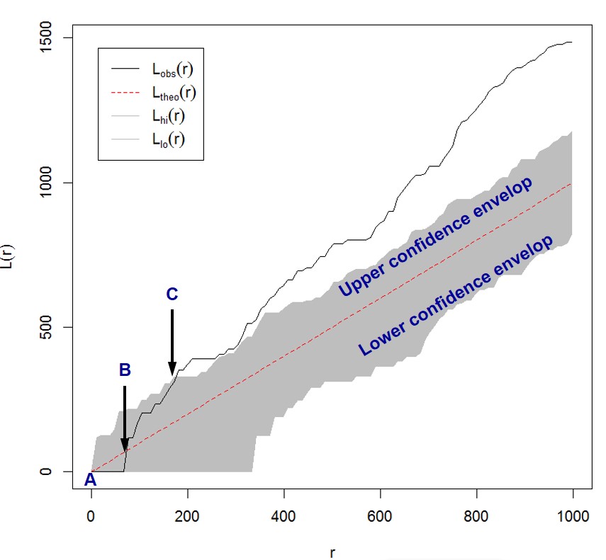] --- ### The L function (Besag 1977) .pull-left[ .large[ The modified L function 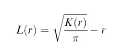 - L(r)>0 indicates that the observed distribution is geographically concentrated. - L(r)<0 implies dispersion. - L(r)=0 indicates complete spatial randomness (CRS). ]] .pull-right[ 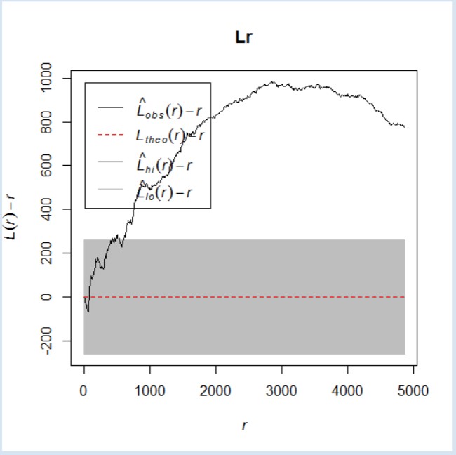] --- ## Kernel density estimation (Silverman 1986) .large[ - A method to compute the intensity of a point distribution. .pull-left[ - The general formula: ] .pull-right[ - Graphically ] ] --- ### Kernel density estimation: simple computation .center[ ] --- ### The kernel functions .center[ ] --- ### Fixed bandwidth .pull-left[ .large[ - Might produce large estimate variances where data are sparse, while mask subtle local variations where data are dense. - In extreme condition, fixed schemes might not be able to calibrate in local areas where data are too sparse to satisfy the calibration requirements (observations must be more than parameters). ]] .pull-right[ 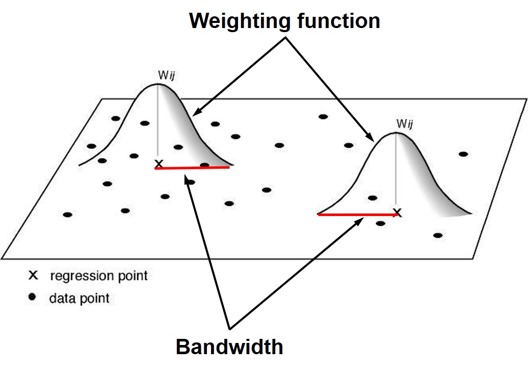] --- ### Adaptive Bandwidth .pull-left[ .large[ Adaptive schemes adjust itself according to the density of data: - Shorter bandwidths where data are dense and longer where sparse. - Finding nearest neighbors are one of the often used approaches. ]] .pull-right[ 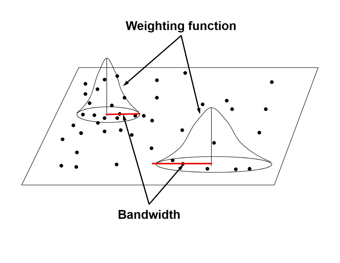] --- # References - [Chapter 11 Point Pattern Analysis](https://mgimond.github.io/Spatial/point-pattern-analysis.html) of **Intro to GIS and Spatial Analysis**. Section 11.2, 11.3, 11.3.1 and 11.4 - GIS&T Body of Knowledge [AM-07-Point Pattern Analysis](https://gistbok.ucgis.org/bok-basic-page/welcome-gist-body-knowledge) - GIS&T Body of Knowledge [AM-08-Kernels and Density Estimation](https://gistbok.ucgis.org/bok-topics/kernels-and-density-estimation) - [Analyzing Patterns in Business Point Data](https://www.directionsmag.com/article/3289), Directions Magazine March 17, 2005. - O’Sullivan, D., and Unwin, D. (2010) **Geographic Information Analysis**, Second Edition. John Wiley & Sons Inc., New Jersey, Canada. Chapter 5-6. - Baddeley A., Rubak E. and Turner R. (2015) **Spatial Point Patterns: Methodology and Applications with R**, Chapman and Hall/CRC.